On the Gaussian Assumption
Is the Gaussian (i.e. normal) distribution tenable?
We recently documented likelihood ratios for individual print pairs in black box studies: Busey T, & Coon, M. Not all Identification Conclusions are Equal: Quantifying the Strength of Fingerprint Decisions. In press, Forensic Science International. pdf. Also see link to Presentation
This paper is important because it demonstrates that for many casework-quality pairs (ones that a majority of examiners with make an identification on) can have strengths of evidence that do not support a phrase such as “Identification”. We often see likelihood ratios in the range of 100-1000, which is much less than is typically associated with a term like “Identification” which is often interpreted by laypersons to mean the exclusion of all others.
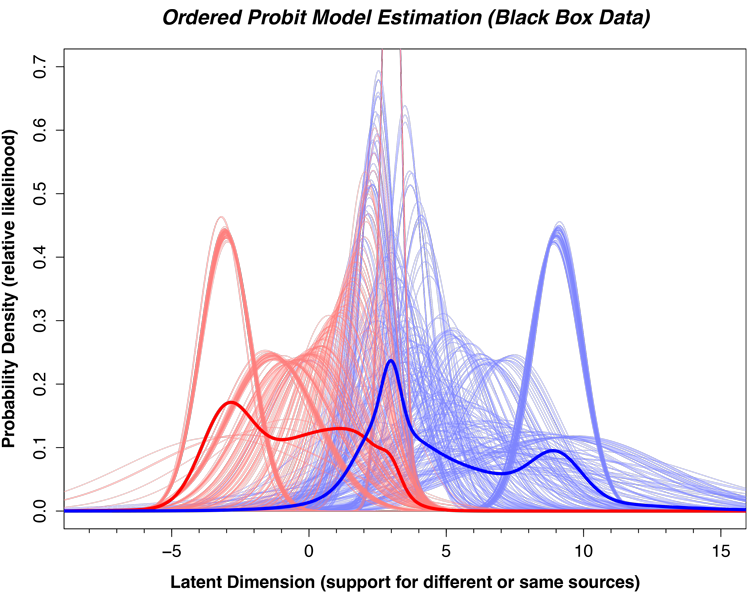
A central assumption of the approach is the use of an ordered probit model, which often includes the assumption of a Gaussian (i.e. normal) latent distribution. Imagine an underlying evidence axis (such as the one in the figure above) that goes from the most support imaginable for the different sources proposition on the left, to the most support imaginable for the same source proposition on the right. Each comparison will have some value along this dimension to each examiner, and when, say, 40 examiners all complete this comparison in a black box study we can summarize these values using a normal distribution. The ordered probit model uses the counts of the different responses (Exclusion, Inconclusive, and Identification) to infer the mean and standard deviation of this underlying distribution.
To compute likelihood ratios, we take the ratio of combined mated and nonmated distributions at each location along the latent axis. This is equivalent to the height of the thick blue curve divided by the height of the thick red curve at every location along the latent axis. The problem comes when we use the tail of the nonmated distribution to estimate the denominator of the likelihood ratio (the right-hand side of the thick red curve above). We don’t have much data in these tails, so how do we know if this assumption is correct?
There are several pieces of evidence that suggest that our model’s assumptions are tenable.
The Gaussian curve has become the default curve with a great deal of empirical support
This argument has been advanced by John Wixted, who is widely known in the psychology literature for his work on eyewitness identification and mathematical modeling (click the reference for the article).
He argues that the Gaussian assumption has been used since Fechner in 1860, Thurstone in 1927, and John Swets in signal detection theory in 1953/54. It is widely used in signal detection theory to model psychological data in perception, memory, attention, and decision making.
The big reason that the Gaussian distribution is so popular is that it tends to occur in situations where lots of small decisions contribute to the outcome. Think of human height, which is the archetypal example of a normal distribution. A person’s height is determined by many genes contributed by both parents and mixing in complex ways. Diet and nutrition also play a role, as well as the health of the mother during pregnancy. All of these little decisions or outcomes contribute to the final adult height, some of which push the adult height higher and some lower. It is true that there are no negative heights, nor are there infinite heights, but this extreme tail behavior is not disruptive enough to reject the utility of the normal distribution as a tool to summarize human height.
Comparisons are the same way: Each examiner will rely on slightly different image features, and have different backgrounds. Because of this they will tend to distribute themselves along the latent axis and arrive at slightly different values. This distribution is what the normal curve is summarizing.
It is entirely possible that the examiner decision is not uni-dimensional, because the information that leads to an exclusion might be different than an identification. The ordered probit model is a summary of these final evidence values, not a model of how to compare prints. An extreme example is when a few examiners erroneously exclude an otherwise easy comparison that the remainder of the examiners correctly ID. While this happens, and can lead to the occasional trade-off between the mean and standard deviation values, these effects are small relative to the overall differences in mu values. These events also typically occur on prints that are fairly easy, but illustrate that a more complete model than the ordered probit model would require some sense of which impressions tend to produce erroneous exclusions and why. Perhaps these have a lack of a clear core or delta to start with and lead to misalignments.
However, just because the comparison process is multi-dimensional does not mean that the final value cannot be on a single dimension. After all, most conclusion scales tend to have a single dimension ranging from Exclusion to Identification. Sometimes the inconclusives are given different explanations (e.g. insufficient minutiae vs no overlap), but procedurally the scale is treated by the forensic consumer on a single dimension, usually one of inculpatory vs exculpatory.
The likelihood ratios are robust to any monotonic transformation of the latent axis
Even if the normal distribution was incorrect, the likelihood ratios are a function of the ratio of the mated and nonmated curves at each value of the latent distribution. If we were to take the log of the mu values (rescaling the latent axis in the figure above) it would not change the ratio between the blue and red curves. The only approach that might affect the likelihood ratios would be to assume that only the nonmated comparisons have right tails that are cropped by some unknown mechanism. This would sharply reduce the height of the thick red curve in the region of around 4-8 on the latent axis, improve the likelihood ratios. However, this proposal assumes we know ground truth and can selectively crop just those curves. If all curves are cropped or skewed in the same way, this is equivalent to the rescaling argument above, and therefore would not change the likelihood ratios.
The area under the nonmated curve is approximately correct
One way to demonstrate that the area under the right tail of the red curve is approximately correct is to consider the area under the right tail relative to the error rates in black box studies. Recall that the erroneous identification rate in the Noblis/FBI black box study was about .001, or 0.1%. This percentage comes from nonmated pairs that behave similarly to mated pairs that receive majority-ID decisions. In the graph below, we plot the cumulative area under the two thick curves to the right of each value along the latent axis (abscissa). Note that in the range of where the image pairs become approximately casework-like, the area under the thick red curve in the image at the top of the page becomes approximately equal to the error rate in the Noblis/FBI black box study.
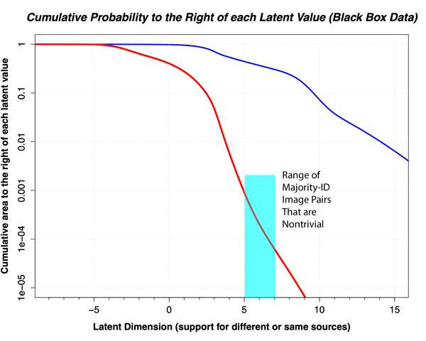 If anything, the area drops to 0.01% or below, suggesting that our nonmated curve might even be too low. If that were the case, the likelihood values we estimate would be too large and the actual values much lower. Thus we see no evidence that our estimate of the right tail of the nonmated distribution is too large, and might not be large enough.
All other assumptions give lower likelihood ratio values
In the original paper, we tried alternative distributions that are typically used as alternatives to summarize latent distributions. These include the Student’s t distribution, which is typically used to model outliers. This might be appropriate for situations where most examiners ID a comparison, but a few exclude. However, this model produced likelihood ratios that were about 2% lower than with the normal distribution despite a value of 5 for the normality parameter. Thus, even with extremely fat tails the likelihood values did not improve. This is to be expected: Fatter tails just push more area from the nonmated distribution into the region of about 5-7 on the latent axis, reducing the likelihood ratios relative to the Gaussian distribution.
While it is possible that there is some other distribution that might produce larger likelihood values, most distributions that reasonably occur in nature have fatter tails than the Gaussian.
Is the 3-conclusion scale too coarse to accurately measure larger likelihood ratios?
One possible explanations for modest likelihood ratios is that the coarse 3-category scale used by examiners does not accurately measure the underlying distribution. Our analysis of the Busey et al (2022) data in the paper did not suffer from that issue, but also was not a true black box study. To address this concern, we conducted a reanalysis of the Noblis/FBI black box data but included difficulty as part of the scale. We grouped Very Difficult and Difficult together to create a “Difficult ID” category, and the remainder of the difficulty statements to create an “Easy ID” category. We did the same thing for the Exclusions.
Although the model has additional categories for Identification and Exclusion, the likelihood ratios were almost identical to those from the traditional 3-category scale. This demonstrates that the modest likelihood ratio values in the published study are not a function of the coarse scale used in the original Noblis/FBI black box study.
Conclusions
The Gaussian (normal) distribution assumption of the ordered probit model has a long history in science, both in psychology and engineering. It is supported by the observation that individual measures that might not be normally distributed become very quickly normally distributed when combined together. Given that the final decision of a comparison is the result of many little steps (including multiple eyemovements as well as different experiences by examiners), the underlying distribution is very likely to be approximately Gaussian distributed.
There is very little evidence for other distributions producing higher likelihood ratios, and assumptions that some distributions can be arbitrarily cropped are not logically tenable. Thus, until a demonstration of a better underlying distribution is offered, the likelihood ratios computed based on the Gaussian distribution remain the most reasonable estimate of the strength of evidence of comparisons in the pattern comparison disciplines.
January 9, 2023